Uni-QSAR

Introduction

QSAR, short for Quantitative Structure-Activity Relationship, is a technique that uses mathematical models to predict a compound's activity based on its structure. By combining historical data with AI technology, QSAR establishes links between molecular structures and their corresponding properties. This approach enables researchers to make informed and efficient predictions about specific groups of molecules. QSAR is extensively used in drug design, environmental toxicology, and chemical safety assessment. The process involves gathering and organizing data on molecular structures and their activities, choosing and extracting molecular descriptors, developing statistical models, and evaluating the models' predictive accuracy.

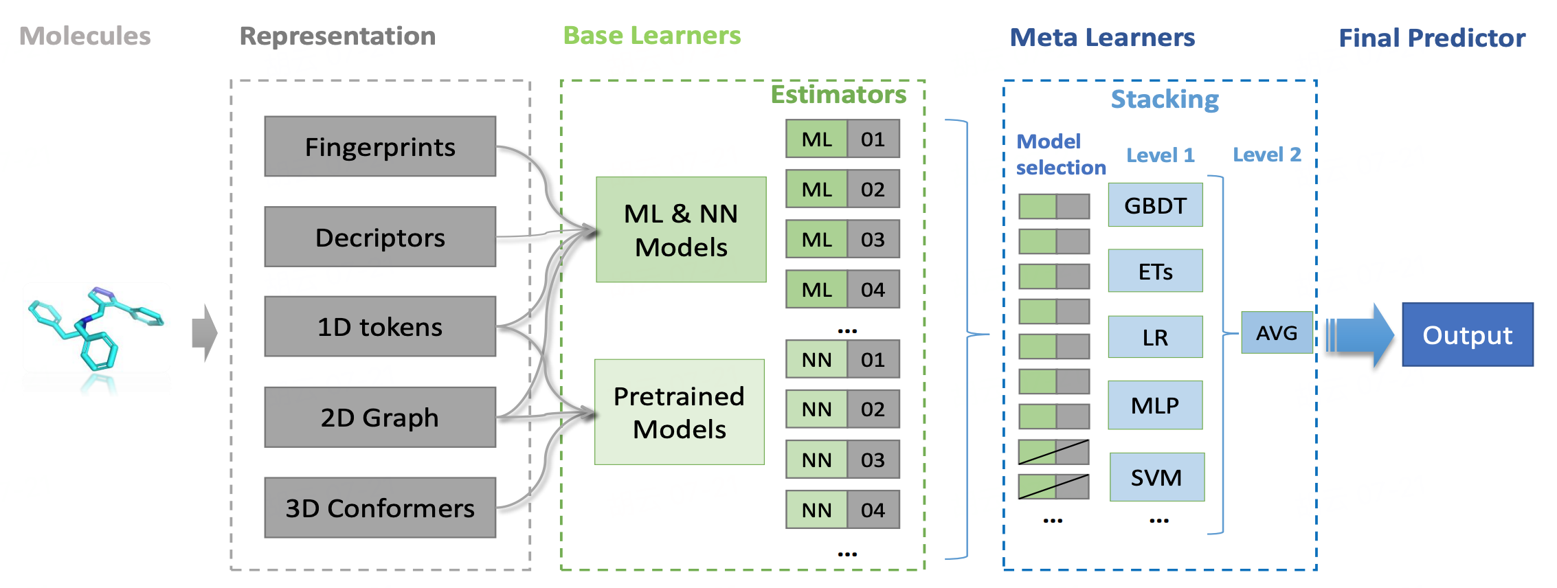
Uni-QSAR is an automated molecular property prediction tool, developed by our team based on the Uni-Mol model. This tool streamlines the process of modeling quantitative relationships between chemical structures and their target attributes. Uni-QSAR module is embeded on the Hermite platform, where users can input molecular formulas in SMILES format and provide data on molecular activity or properties. The system then builds QSAR models using machine learning and deep learning techniques. These models are capable of predicting the activities of new molecules, offering a powerful resource for research and development.

In this tutorial, you will build a sweet and non-sweet classification model based on Uni-QSAR, using data from the article "BitterSweet: Building machine learning models for predicting the bitter and sweet taste of small molecules" [2] .

The classification dataset used in this tutorial are as follows:

Sweetness_test.csv

Sweetness_training.csv

Sweetness_prediction.csv

1. Building a QSAR Model

1.1 QSAR Modeling Entry

Go to "Function" → "Molecular Recommendation" → "Uni-QSAR".

In the pop-up window, select "Build Model".

1.2 Uploading Dataset and Setting Parameters

Click "From File" at "Select Data for Training" and upload the "Sweetness_training.csv" file.

Note: Up to 1 million rows allowed.

Choose " Classification " at "Task".

Type	Meaning
Regression	Continuous property data required for prediction
Classification	Non-continuous property data; binary classification and multi-label classification are supported.

Select "Scaffold" for the cross-validation split method for the training dataset at "Cross Validation split".

Random	Scaffold
Random split	Split the training dataset based on the molecular scaffold (molecular structures with ideal properties). Recommended data splitting method for more efficient splitting and training.
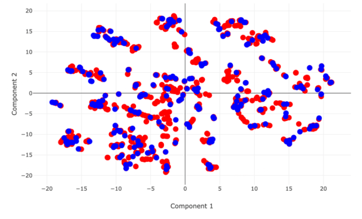PCA distribution map of two datasets when choosing “Random”	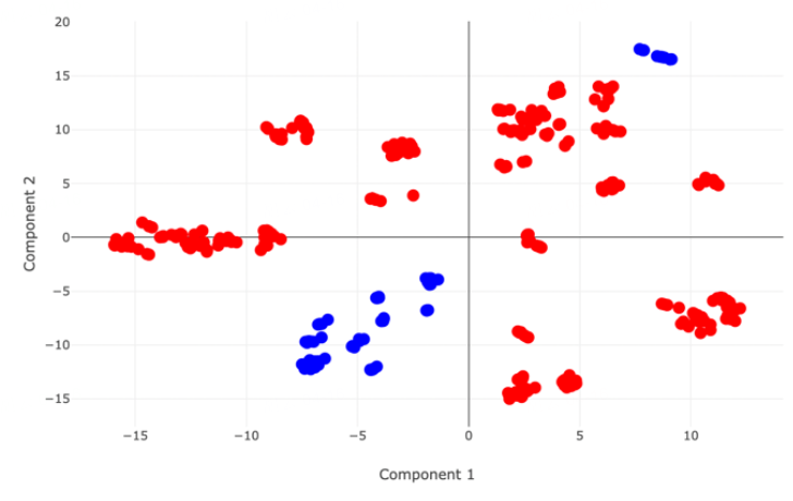PCA distribution map of two datasets when choosing “Scaffold”

Go to "Select Test Set" and choose "Select Data for Test" → click "From File" to upload the file "Sweetness_test.csv".

Test set upload method	Meaning
Split from Training Data	A certain percentage (%) of the training dataset is used as a test set
Select Data for Test	Upload local test set

You can keep the default task name or enter a new one, then lick "Next" to proceed to the next step.

1.3 Selecting Properties and Submitting the Task

Select the property that needs to be trained for prediction under "Properties Setting" -> Confirm the calculation cost under "Calculation" - > Click "Submit" to submit the task.

Note: In this case, sweetness is marked as 1 and non-sweetness is marked as 0.

2. Model Performance Evaluation

2.1 Viewing Uni-QSAR Modeling Results

Go to "Job" → Find the required task → Click "Show" in the "Operation" column to show the result of the task.

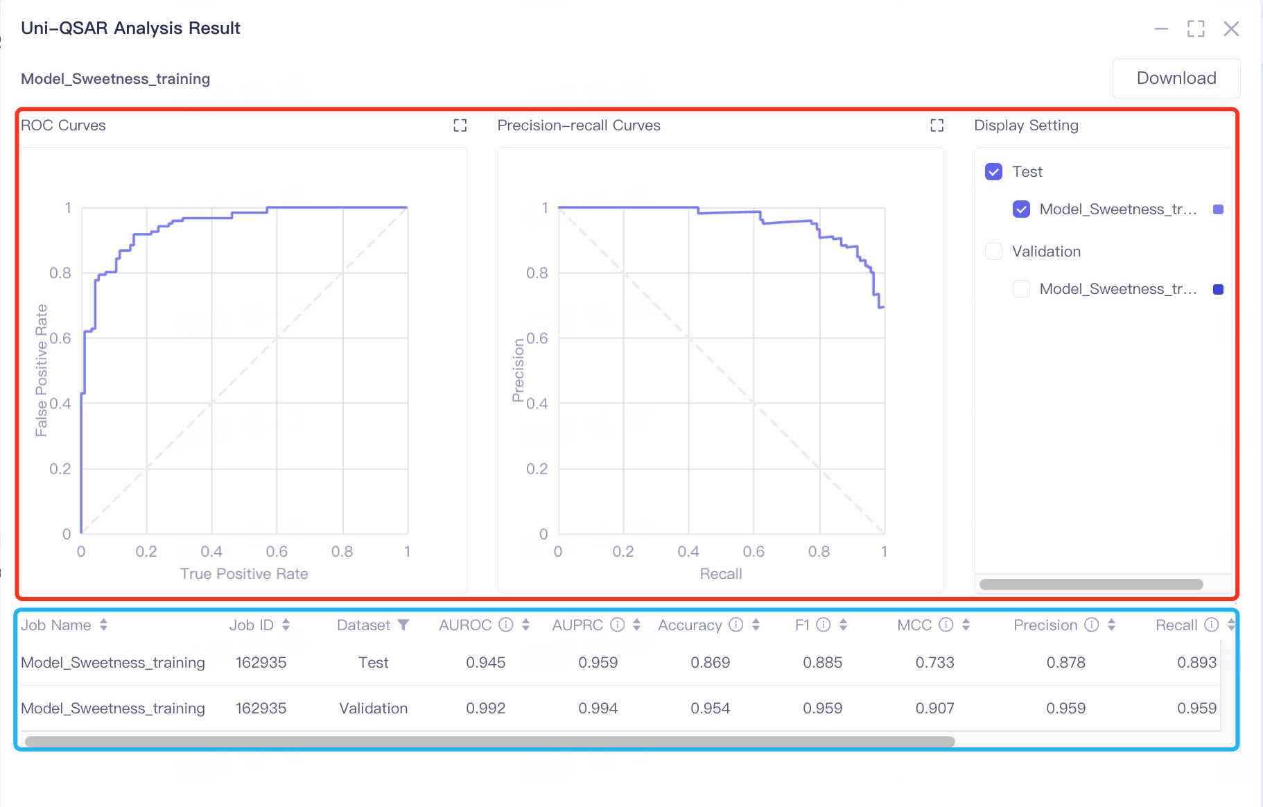
The results are divided into two parts, some charts (in the red box) and a table (in the blue box).

The results are presented in two sections: charts within a red box and a table in a blue box. The model's predictive performance is primarily gauged by AUROC and AUPRC values. In the validation and test sets, AUROC scores of 0.992 and 0.945 respectively indicate the model's strong ability to classify sweetness and non-sweetness. The AUPRC scores, 0.994 in the validation set and 0.959 in the test set, highlight the classifier's effectiveness in predicting positive instances of sweetness.

Additional metrics like Accuracy, F1, MCC, Precision, and Recall further assist in assessing the model's performance. High scores in these metrics suggest the model's excellent capability in distinguishing between sweet and non-sweet tastes.

Classification model
Evaluation metrics	Meaning	Value range
AUROC	Area Under the Receiver Operating Characteristic Curve (AUROC) represents the classifier's ability to correctly distinguish between positive and negative samples. The ROC curve is plotted with the True Positive Rate (TPR) on the y-axis and the False Positive Rate (FPR) on the x-axis, based on different thresholds of the classifier.	The value ranges from 0 to 1. The higher the value, the better the performance of the classifier. AUROC is better to use when the categories are balanced.
AUPRC	Area Under the Precision-Recall Curve (AUPRC) represents the performance of the classifier in predicting positive instances. The Precision-Recall curve is plotted with Recall (also known as the True Positive Rate) on the y-axis and Precision on the x-axis, based on different thresholds of the classifier.	The value ranges from 0 to 1. The higher the value, the better the performance of the classifier. It is better to use AUPRC when the categories are extremely unbalanced.
ACC	Accuracy. $ACC= \frac{TN+TP}{TP+FP+TN+FN}$	The value ranges from 0 to 1. The higher the value, the better the performance of the classifier.
F1	$F1= \frac{2×Precision×Recall}{Precision+Recall}$	The higher the value, the better the performance of the classifier.
MCC	MCC is essentially a correlation coefficient that describes the actual classification and the predicted classification. $MCC=\frac{TN × TP - FN × FP}{\sqrt{(TP + FP)(TP+FN)(TN+FP)(TN+FN)}}$	The range of the value is [-1, 1]. When the value is 1, it represents a perfect prediction for the test object. When the value is 0, it indicates that the predicted result is worse than the randomly predicted result. -1 means that the predicted classification is completely inconsistent with the actual classification.
Precision	Precision rate, the proportion of correctly predicted positive samples. $Precision = \frac{TP}{TP+FP}$	The value ranges from 0 to 1. The higher the value, the better the performance of the classifier.
Recall	Recall ,the proportion of positive samples that are predicted to be positive. $Recall = \frac{TP}{TP+FN}$	The value ranges from 0 to 1. The higher the value, the better the performance of the classifier.
Cohen's kappa	The Kappa coefficient is a method used in statistics to evaluate consistency and can be used to evaluate the accuracy of multi-classification models .	The range of the value is [-1, 1]. In practical applications, it is generally [0, 1]. The higher the value of this coefficient, the higher the classification accuracy achieved by the model.
Logistic Loss	Logistic loss is a likelihood estimate of the predicted probability, measuring the difference between the predicted probability distribution and the true probability distribution.	The lower the value, the better.
Note: TN - Number of samples correctly predicted as negative; TP - Number of samples correctly predicted as positive; FN - Number of samples incorrectly predicted as negative; TP - Number of samples incorrectly predicted as positive.
Regression model
Evaluation metrics	Meaning	Value range
MAE	The average absolute value error is calculated by calculating the absolute value of the difference between the predicted value and the true value of each sample, and then summed and averaged. It is used to evaluate the closeness of the predicted results to the true value.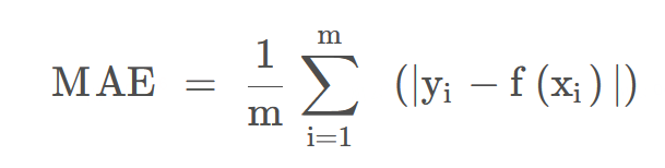	The lower the value, the better the fitting effect.
MSE	The mean squared error (MSE) of a model measures the average of the squares of the errors—that is, the average squared difference between the estimated values and the actual value.	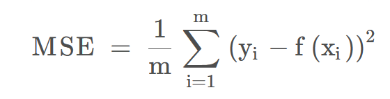The lower the value, the better the fitting effect.
RMSE	The root mean square error is the square root of the mean square error.	The lower the value, the better the fitting effect.
R²	Coefficient of determination. R² is a measure of the goodness of fit of a model.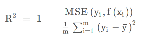	The determinate coefficient value is between - ∞ ~ 1. The closer to 1, the better the prediction effect of the model, and the lower the value, the worse the performance of the model.
Spearmanr	The Spearman rank-order correlation coefficient is a nonparametric measure of the monotonicity of the relationship between two datasets. It is a non-parametric measure used to evaluate the relationship between two variables that do not follow the Normal Distribution, or when the relationship between variables is non-linear.	Values range from -1 to 1, with 0 indicating no correlation, 1 indicating a perfect positive correlation, and -1 indicating a perfect negative correlation.
Pearsonr	Pearson correlation coefficient measures the linear relationship between two datasets.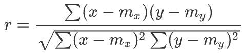	The range is between -1 and + 1, where 0 indicates no correlation, and the correlation of -1 or +1 indicates a precise linear relationship.

2.2 Download Uni-QSAR Modeling Results

Go to "Job" → Find the required task → Click "Download" in the "Operation" column to retrieve the results.

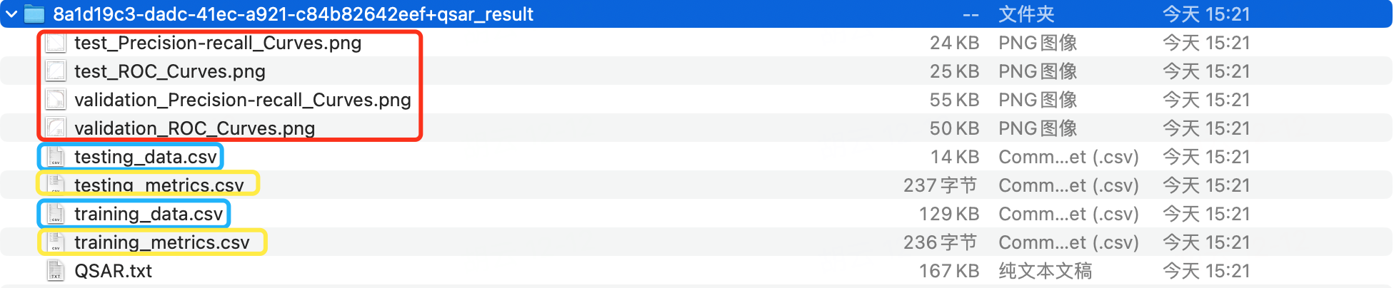
The downloaded .zip file contains four types of files.

1. [...].png: Binary classification models produce ROC and PR curves for both validation and test sets. Single-label regression models generate scatter plots of predicted versus actual values.

2. [...]_data.csv: Includes training dataset data (training_data.csv) and test set data (testing_data.csv).

3. [...]_metrics: Consists of cross-validation result files for the training dataset (validation_metrics.csv) and test set results (testing_metrics.csv).

4. QSAR.txt: A log file documenting the modeling process.

3. Prediction Based on a Historical Model

This step involves using a previously trained model to predict if novel molecules are sweet.

3.1 Prediction Entry

In the same project, navigate to the common menu bar on the left and click"Function" → "Molecular Recommendation" → "Uni-QSAR".

A new interface will appear and select "Make Prediction"

3.2 Model Selection and File Upload

To choose a historical model, click on "History Model"

To upload your data, click "From File" and select the "Sweetness_prediction.csv" file from your local storage. Ensure the file format matches that of the training dataset, though this file may only contain column headers without data.

Keep the default job name or enter a new one.

Click "Submit" to start the prediction.

4. Check results

Navigate to "Job" → Search for "Prediction_Sweetness_prediction" → Click "Download" in the "Operation" column to download the results.

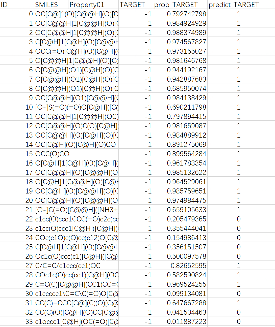
The downloaded .zip file includes two files: "predicted_data.csv", which contains the prediction results, and "QSAR.txt", a log file.

Note: In "predicted_data.csv", the "predict_TARGET" column indicates the molecular sweetness prediction, with 1 for sweetness, and 0 for non-sweetness; the "prob_TARGET" column shows the predicted probability of molecular sweetness.

5. References

[1] Gao Z, Ji X, Zhao G, et al. Uni-QSAR: an Auto-ML Tool for Molecular Property Prediction. arXiv preprint arXiv 2304, 12239 (2023). https://doi.org/10.48550/arXiv.2304.12239

[2] Tuwani, R., Wadhwa, S. & Bagler, G. BitterSweet: Building machine learning models for predicting the bitter and sweet taste of small molecules. Scientific Reports 9, 7155 (2019). https://doi.org/10.1038/s41598-019-43664-y